Chapter 3 Designing the Study

3.1 Basic steps in designing your study

You have chosen your research question and formulated a hypothesis. You have collected and screened relevant literature on the topic. Now you need to decide on your research design. Are you planning to uncover associations, or do you want to examine a causal relationship between your variables of interest (Pearl 2009; Pearl, Glymour, and Jewell 2016)? We will focus on investigating causal relationships and analyzing counterfactual situations. To translate direct observations in data to investigate cause-and-effect relationships, you need to rely on a workable model that describes the elements and relationships of interest reflected in your hypothesis. It is strongly recommended that you first describe the causal structures of the elements that you are studying, including any other observed or unobserved structures that may disturb the cause-and-effect relationship under investigation.

The three rungs of the ladder of causality can be shortly described as adapted from Sobolev Spaces

Rung	Queries and targets
Level 1: ASSOCIATIONS	Query: Is the outcome more common in one treatment group than the other? Target: Difference between groups
Level 2: EFFECTS OF CAUSES	Query: How would outcomes differ if treatment groups were made up of the same subjects (individuals, neighborhoods, firms)? ; Target: Average treatment effect
Level 3: CAUSAL ATTRIBUTION - COUNTERFACTUALS
CAUSATION	Query: How likely is it that treatment is necessary and sufficient cause of the outcome?; Target: Necessary and sufficient causes
MEDIATION	Query: What part of the average treatment effect is not mediated by other treatment outcomes?; Target: Natural direct effect
️PERSONALIZED EFFECT	How prevalent is responding differently to different treatments?; Target: The probability of causation bounds

Two approaches may be used to describe the causal relationships and the estimable effects that you may identify as part of your research question:

1. Potential outcomes framework (PO-framework)
2. Directed acyclic graphs (DAG)

Both approaches are the powerhouses to performing empirical analyses to specify a) the effects that you aim to identify and b) the structural relationships between the concepts (dependent variables, variables of interests and confounders) under evaluation and c) whether your results allow for causal inference given your data. Both approaches are powerful and comprehensive. We keep this section short and refer to important resources in the field below.

The design of your study will depend on the causal model that suggests which effects are estimable, given that there are suitable data to empirically identify the effect. Consider that you describe cause-and-effect relationship first, assess how it is estimable (that means that you ask the question “Can you infer a causal effect from your data?”) and then investigate the effect by direct observations using secondary data.

3.1.1 Potential Outcomes Framework

The potential outcomes framework uses the potential values of the outcomes given a certain treatment (Abadie and Cattaneo 2018) to describe the causal parameters that you aim to identify in your empirical analysis and the type of effect. The PO-framework is particularly suited for evaluating the effect of policies (governmental, firm policies). In short, you would like to compare outcomes given a subject (individual, firm, region) has received a treatment to the outcomes when the subject has not received a treatment. The difference between the two will tell you the treatment effect from having received the treatment or policy under investigation by defining potential and realized outcomes. Using the potential outcomes framework helps you to specify and assess whether you can conclude that your estimands are coming from a population where the treatment has been randomly assigned to subjects.

In the most simplest notation, consider that there is a value of the treatment by the (random) variable \(X\), also often denoted as \(W\) or \(D\). We largely borrow from Abadie and Cattaneo (2018)’s annotation. Consider that \(X\) has two values \(1\) which stands for that a subject has received a treatment, and \(0\) which stands for that the individual has not received the treatment. The goal is to investigate the effect of changes in \(X\) on some observed outcomes variable, denoted as \(Y\). \(Y_1\) represents the potential value of the outcome when the value of the treatment variable \(X\) is set to \(1\). \(Y_0\) represents the potential value of the outcome when the subject does not receive the treatment. The causal effect of the treatment can be represented by the difference in potential outcomes, \(Y_1-Y_0\). The potential outcomes and the value of the treatment define the observed outcome

\(Y=XY_1+(1-X)Y_0\)

Note that we typically cannot observe both potential outcomes in the same subject which refers to as the fundamental problem of causal inference. To be able to make causal statements, we need to make additional assumptions to be able to estimate the average treatment effect (ATE), i.e.

\(\tau_{ATE}=E[Y_1-Y_0]\)

This is a very short representation of the PO-Framework and we refer the reader for the additional identifying assumptions to the resources box below.

3.1.2 Directed Acyclic Graphs

One way of describing your causal structure is by describing causal relationship in directed acyclic graphs (DAG). A DAG is a systematic representation of a causal relationship between two (or more) variables (\(X\) and \(Y\)) with a focus on minimizing statistical bias by potential confounding variables (\(Z\)). It is recommended to do this step before data collection. That way, you avoid collection of data that may not be needed. You also avoid forgetting variables that are necessary for causal effect identification. And you may check for so-called bad controls that may bias your estimates.

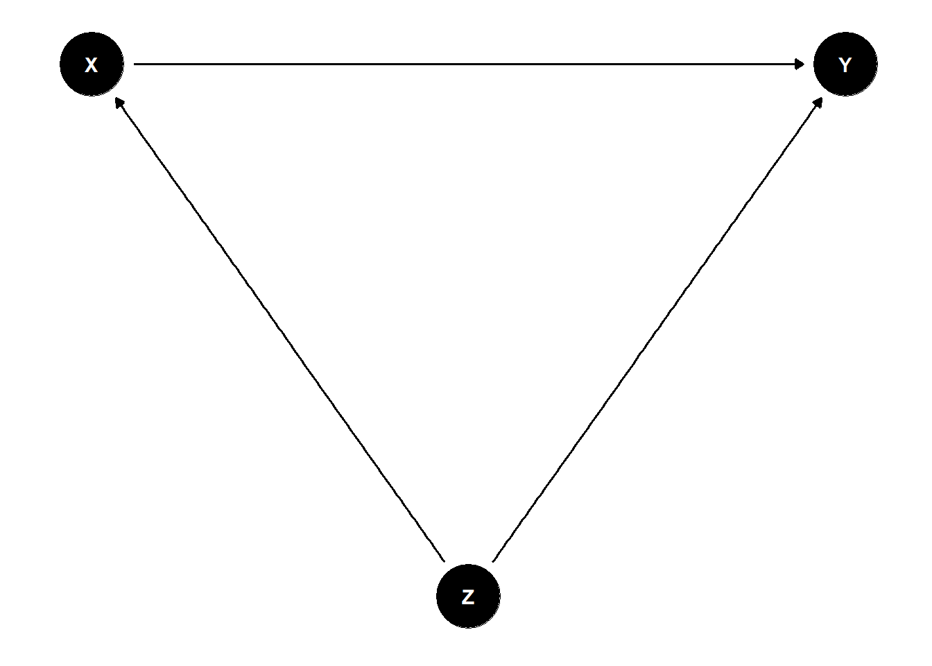
Figure 3.1: Directed Acyclic Graph

3.1.3 Develop a causal model and identify estimable effects

We focus on study designs that use secondary data with the aim to identify the magnitude of effects of causal relationships between a variable of interest \(X\) and a certain outcome \(Y\), controlling for potential confounders \(Z\). Note that there is extensive literature and guidance about designing and performing causal inference studies, some of which we guide you to below. We will highlight the most important elements and point to the relevant resources.

Consider the subsequent steps as an iterative process, allowing that not all data you may need to estimate effects of your causal model will be readily available. Some elements will remain unobserved. For others, you may need to find proxies.

You should specify a causal model that describes the relationships between the elements that you are studying. This causal model will help to identify an empirical model by defining your main relationship of interest.

Generally speaking, you need to specify your

• main outcome variable of interest (\(Y\))
• main independent variable of interest (\(X\))
• other independent variables (confounders of the effect of \(X\) on \(Y\)), that means any additional \(Z\)’s
• unobserved variable (\(U\))

You need to think about how these concepts can be measured and what the relationships between these concepts are.

3.1.4 Develop the empirical strategy to investigate causal effects

After you have specified your causal model, ask yourself how you can capture the causal relationship between \(X\) and \(Y\)? In other words, can you apply an appropriate research design that can accommodate you in determining causality with the data at hand? Use the potential outcomes framework notation to describe the types of effects you aim to identify.

Following the classification by Matthay et al. (2020), that means performing, for example, a

• Randomized Controlled Trial (RCT): this is be the ideal world case where we randomize treatments to study effects. You actively assign a treatment to subjects by chance.

Most secondary data are collected retrospectively and thus will not allow performing a RCT as you will not be able to manipulate treatment assignment. You will not be able to randomly assign subjects ahead of time, such that you typically need to search for the best available quasi-experiment to identify treatment effects using a

• Confounder Control Study

  • Regression adjustment
  • Matching techniques
  • Simulation
  • Random or Fixed effects regressions
  • Instruments
  • Regression discontinuity design (RDD)
  • Difference-in-differences (DiD) analysis
  • Instrumental variable (IV) approach

• Any other method such as synthetic control groups, structural equation models, causal machine learning

Think about what type of treatment effect you are investigating in your causal analysis. The treatment effect is the average (across the population or across some subpopulation) change in outcome (\(Y\)) that results from a change in a covariate (the treatment \(X\)) (Lewbel 2019).

Common types of treatment effect parameters are

• average treatment effects (ATE)
• average treatment effects on the treated (ATT or ATET)
• marginal treatment effects (MTE)
• local average treatment effects (LATE)
• quantile treatment effects (QTE)
• intention to treat effect (ITT)

3.1.5 Investigate suitable source data

You need to find and collect suitable data to populate your causal model. This might take some time, and not all of the variables can be found in one dataset. Frequently, different data sources need to be collected and combined. You need to decide on what aggregation level you need to conduct your analysis to estimate the cause-and-effect relationships postulated, for example, individual (patient, student), organization (hospital), regional (country, state). Given that, you need to identify appropriate data sources that contain your variables of interest at the given aggregation level.

When searching for the data sources, you can turn to already existing datasets specifically designed for scientific use, for example, surveys (NAMCS, CPS, NLSY, HILDA, RLMS, KiGGS); panels (for example, GSOEP, SHARE, HRS, ELSA); censuses (e.g., Microcensus).

Some data are available from statistical offices (Eurostat in the European Union, DESTATIS for Germany), private companies (health insurances), Social Media and App-based data (Mappiness, Fitbit, Facebook, Twitter, WayBetter) or governmental and non-governmental institutions (European Medicines Agency, Food and Drug Administration). Sometimes you have to hand-collect and digitize the necessary data, for example, from historical documents, data from governmental and non-governmental agencies, commercial providers and library search engines, archives; download statistical tables from INKAR’s (INKAR - Indikatoren und Karten zur Raum- und Stadtentwicklung) or Unemployment Agency’s websites. Therefore, you need to plan whether and how these can be accessed and how much time is needed for extraction. Consider automated tools like scraping.

3.2 Resources box

3.2.1 Key terminology in causal inference based on Matthay et al. (2020)

• Causal model: A description, most often expressed as a system of equations or a diagram, of a researcher’s assumptions about hypothesized known causal relationships among variables relevant to a particular research question.
• Treatment, exposure, or independent variable: The explanatory variable of interest in a study. Some also describe this as the “right-hand-side variable”.
• Outcome, dependent variable, or left-hand-side variable: The causal effect of interest in a research study is the impact of an exposure(s) on an outcome(s).
• Potential outcome: The outcome that an individual (or other unit of analysis, such as family, neighbourhood, physician) would experience if his/her treatment takes any particular value. Each individual is conceptualized as having a potential outcome for each possible treatment value. Potential outcomes are sometimes referred to as counterfactual outcomes.
• Exogenous versus endogenous variables: These terms are common in economics, where a variable is described as exogenous if its values are not determined by other variables in the causal model. The variable is called endogenous if it is influenced by other variables in the causal model. If a third variable influences both the exposure and outcome, this implies the exposure is endogenous.

3.2.2 Openly available textbooks and resources on econometrics with a causal inference focus

• Causal Inference: The Mixtape by Scott Cunningham
• What If by Jamie Robin and Miguel Hernan
• The Effect: An Introduction to Research Design and Causality by Nick Huntington-Klein
• How Do We Know if a Program Made a Difference? A Guide to Statistical Methods for Program Impact Evaluation by MEASURE Evaluation
• Open Source Economics Basics to microeconometric methods
• Introduction to Econometrics using R by Christoph Hanck
• Econometrics by Bruce E. Hansen
• Mastering Econometrics by Joshua Angrist
• Differences-in-Differences design, Health Care Policy Science Lab
• Statistical Tools for Causal Inference by the SKY Community

3.2.3 Ladders of causality and directed acyclic graphs

• A more comprehensive overview of causal paths is provided by Nick Huntington Klein
• A tool to draw Directed Acyclic Graphs (DAGs) is DAGitty
• Pearl’s Causal Epistemology

3.2.4 Potential outcomes framework notation

• Causal Inference Chapter in Health Services Research Methods I
• The fundamental problem of causal inference

3.3 Checklist to get started with designing your study

• Describe your outcomes, variables of interest, confounders and potentially, unobserved variables
• Identify at which rung in the ladder of causality you will be investigating your research question
• Get familiar with the foundations of your selected identification and estimation strategy
• Identify appropriate secondary data sources that populate your causal model. Ensure that access is granted within the given timeframe of your project
• Challenge your identifiability assumtions
• Refer back to similar empirical studies and reflect on their design and identification strategy

3.4 Example: Hellerstein (1998)

The identified research question and the hypothesis that physicians are more likely to prescribe generics to patients who do not have insurance coverage for prescription pharmaceuticals can be modelled with the help of a directed acyclic graph (DAG).

#  set theme of all DAGs to `theme_dag()`--> minimalist 
library(ggdag)
theme_set(theme_dag())

Hellcoords <- list(
    x = c(Y =5, P=1, C=1, X=2, R=3,XP=4),
    y = c(Y =0, P=0, C=-1, X=-1, R=-1,XP=-1))


Hellersteindag <- dagify(Y ~ P + C + X + R + XP,
                         P ~ X + XP + C + R,
                         labels = c("Y" = "Prescription of Generic Drug",
                                    "P" = "Patient's Insurance Status",
                                    "C" = "Drug Prices (Class Fixed Effects)",
                                    "X" = "Patient Characteristics",
                                    "XP" = "Practice Characteristics",
                                    "R" = "Region"),
                         exposure = "P",
                         outcome = "Y", coords=Hellcoords)

#ggdag(Hellersteindag, text = TRUE, use_labels = "label")

ggdag_classic(Hellersteindag)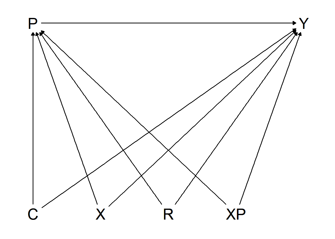

Figure 3.2: Directed Acyclic Graph, Hellerstein (1998)

Figure 3.2 points out the effect of interest as well as potential confounders. Hellerstein sets up an observational, retrospective analysis of secondary data, including patient and physician characteristics. The goal of the analysis is to identify a causal effect of the patient’s insurance status (independent variable, \(P\)) on the prescription of a generic over a trade-name drug (dependent variable, \(Y\)). As the physician’s prescription decision is prone to involve information imperfections and agency problems, the empirical model needs to control for physician-specific effects among other possible influencing factors, generally represented by confounders \(Z\), and specifically by drug prices \(C\), patient characteristics \(X\), practice characteristics \(XP\) and the region \(R\). Another factor Hellerstein is concerned about is random variation at physician level in the choice between generic and trade-name drugs.

The study is based on data from the National Ambulatory Medical Care Survey (NAMCS) 1991, provided by the Centers for Disease Control and Prevention (CDC). The NAMCS is a national sample survey administered by the National Center for Health Statistics. The NAMCS data contain all actions taken by a physician in this period. NAMCS allows controlling for physician-specific behavior that is necessary to draw conclusions of our estimand – the effect of the patient’s insurance status.

The confounder control study design chosen by Hellerstein (1998) uses a random effects probit specification at physician level to estimate the effect of insurance status on generic compared to trade-name drug choice. This includes the outcome variable (\(Y\)), a binary variable, which indicates whether a patient has been prescribed a trade-name or a generic drug. \(Y\) takes the value \(1\) if a generic drug or the value \(0\) if a trade-name drug was prescribed. Of interest is the causal effect of the patients’ insurance types that include Medicare, Medicaid, HMO/prepaid and private insurance. Other independent variables included in the analysis for the purpose of reducing possible bias are the drug class as proxy for prices, patient characteristics (age, gender, race), physician specialist status, the region and the averages of patient characteristics at physician level. The physician-level practice demographics help portraying heterogeneity in the physician’s practice composition, as they contain all patients, including the patients that did not receive any drug prescription.

Note that Hellerstein does not use the potential outcomes notation, but we assume that the variables described as confounders besides the variable of interest \(P\) represent all necessary confounding variables. This assumption can only be informed from theory and cannot be validated using empirical methods.

Hellerstein (1998) specifies the following estimation equation:

\[P(Generic_{ij}=1|C_k,X_i,\overline{P}_j,S_j, R_j,\overline{X}_j,\overline{P}_j)\] \[= C_k\lambda+X_i\beta+C_kP_i\gamma+S_j\pi_1+R_j\pi_2+\overline{X}_j\pi_3+\overline{P}_j\pi_6+v_j+\epsilon_{ij}\]

where

• \(C_k\): drug classes
• \(X_i\): vector of patient demographics
• \(P_i\): insurance categories
• \(S_j\): indicator if a physician is a specialist
• \(R_j\): region
• \(\overline{X}_j\): practice level patient characteristics based on \(X_i\)
• \(\overline{P}_j\): share of patients in each insurance category in a physician’s practice

Contrary to Hellerstein (1998), this equation leaves out indicators for mandatory substitution laws, \(M\) and \(T\), as this information was in confidential data files. Hellerstein describes that she uses a random effects probit specification at physician level, however, the specified equation looks different than the usual random effects specification. You can find more information on random effect models in Huntington-Klein (n.d.).

The choice of the covariates depends on the underlying causal model that is rooted in theoretical considerations. Often you will not find all variables that are confounders directly. Your creativity is needed to find appropriate proxies in the data at hand to account for any relevant possible biases. An example from Hellerstein’s 1998 study design is the need to include prices into the empirical analysis. Hellerstein assumes that physicians are price sensitive. The physicians might not know the true price difference between trade-name and generic drug, but have an expectation of price differences. This poses a potential bias, as the physician might alter her prescription style to these expectations. Prices are not provided in NAMCS such that unobservable price differences are accounted for by including drug class dummy variables. The rationale for drug class dummies is that prices vary across drug classes. Including drug class dummy variables allows capturing variation in the prices of products indirectly.

The empirical specification by Hellerstein uses a random effects probit estimator that is efficient under certain assumptions. The identifiability of the effect of insurance status on generic compared to brand-name products is not explicitly described. The specification of the estimator is described in (Cameron and Trivedi 2005, 705). Note that while random effects estimators are typically used in panel data that use a time dimension, Hellerstein uses multiple observations at drug-class level instead of time dimensions.¹

References

Abadie, Alberto, and Matias D. Cattaneo. 2018. “Econometric Methods for Program Evaluation.” Annual Review of Economics 10 (1): 465–503. https://doi.org/10.1146/annurev-economics-080217-053402.

Cameron, Adrian Colin, and Pravin K. Trivedi. 2005. Microeconometrics: Methods and Applications. Nachdr. Cambridge: Cambridge Univ. Press.

Hellerstein, Judith K. 1998. “The Importance of the Physician in the Generic Versus Trade-Name Prescription Decision.” The RAND Journal of Economics 29 (1): 108–36. https://doi.org/10.2307/2555818.

Huntington-Klein, Nick. n.d. Chapter 16 - Fixed Effects the Effect. Accessed March 1, 2022. https://theeffectbook.net/ch-FixedEffects.html.

Lewbel, Arthur. 2019. “The Identification Zoo: Meanings of Identification in Econometrics.” Journal of Economic Literature 57 (4): 835–903. https://doi.org/10.1257/jel.20181361.

Matthay, Ellicott C., Erin Hagan, Laura M. Gottlieb, May Lynn Tan, David Vlahov, Nancy E. Adler, and M. Maria Glymour. 2020. “Alternative Causal Inference Methods in Population Health Research: Evaluating Tradeoffs and Triangulating Evidence.” SSM - Population Health 10 (April): 100526. https://doi.org/10.1016/j.ssmph.2019.100526.

Pearl, Judea. 2009. Causality. Cambridge: Cambridge University Press. https://doi.org/10.1017/CBO9780511803161.

Pearl, Judea, Madelyn Glymour, and Nicholas P. Jewell. 2016. Causal Inference in Statistics: A Primer. Chichester, West Sussex: Wiley.

---

1. A fixed effects (FE) estimator using physician-level fixed effects and additional specifications could be considered more appropriate to capture the within-physician variation, we do not discuss alternative estimators contrary to Hellerstein’s approach, but concentrate on the initial design.↩